Principles of Quantum Computing
Teaching experiments on quantum computing process
NMR Phenomena and Signals
The most basic NMR experiment is used to observe nuclear magnetic resonance phenomena:
from spinqlablink import SpinQLabLink, ExperimentType, Pulse
from spinqlablink import print_graph

def nmr_signal_experiment():
    """NMR Phenomenon and Signal Experiment"""
    # Connect to device
    spinqlablink = SpinQLabLink("192.168.9.121", 8181, "username", "password")
    spinqlablink.connect()
    spinqlablink.wait_for_login()

    try:
        # Register experiment
        _, exp_para = spinqlablink.register_experiment(ExperimentType.NMR_PHENOMENON_AND_SIGNAL)

        # Set pulse sequence
        exp_para.pulses = [Pulse(path=0, width=40, amplitude=100, phase=90, detuning=0)]

        # Set frequency parameters
        exp_para.freq_h = 37.852105  # Hydrogen resonance frequency
        exp_para.freq_p = 15.322872  # Phosphorus resonance frequency
        exp_para.makePps = True
        exp_para.samplePath = 0
        exp_para.custom_freq = False

        # Run experiment
        spinqlablink.run_experiment()
        spinqlablink.wait_for_experiment_completion()

        # Get and display results
        result = spinqlablink.get_experiment_result()
        print_graph(result["result"])

    finally:
        spinqlablink.deregister_experiment()
        spinqlablink.disconnect()

if __name__ == "__main__":
    nmr_signal_experiment()
Experimental Parameters Analysis
ExperimentType: Select NMR_PHENOMENON_AND_SIGNAL(for details, see:class:spinqlablink.ExperimentType class)
Pulse: Define the pulse sequence and set the path, width, amplitude, phase and frequency offset of the pulse (see:class:spinqlablink.Pulse class for details)
freq_h: Hydrogen resonance frequency (hz) [0- 100M]
freq_p: Phosphorus resonance frequency (hz) [0- 100M]
makePps: Whether to use PPS pulse sequences
samplePath: Sampling path, 0= hydrogen channel, 1= phosphorus channel [0-1]
custom_freq: Whether to use custom frequency [True,False]
Analysis of experimental results
{
    "result":{
        "graph":[
            { # step 0
                "fidRe": [[x,y],...],
                "fidIm":[[x,y],...],
                "fftRe":[[x,y],...],
                "fftIm":[[x,y],...],
                "lorenz":[[x,y],...],
                "fftRe":[[x,y],...],
                "fftIm":[[x,y],...],
                "fftMod":[[x,y],...],
                "fidMod":[[x,y],...],
                "fftFit":[[x,y],...]
            },
            { # step 1},
            ...
            ]
        }
    }
}
- graph: Chart data, including real and imaginary parts. The graph contains 1 step, and each step may contain the following data:
fidRe: FID Real Component
fidIm: FID Imaginary Component
fidMod: FID Modulus
lorenz: Lorenz fitted curve
fftRe: FFT Real Component
fftIm: FFT Imaginary Component
fftMod: FFT Modulus
fftFit: FFT Fit Curve
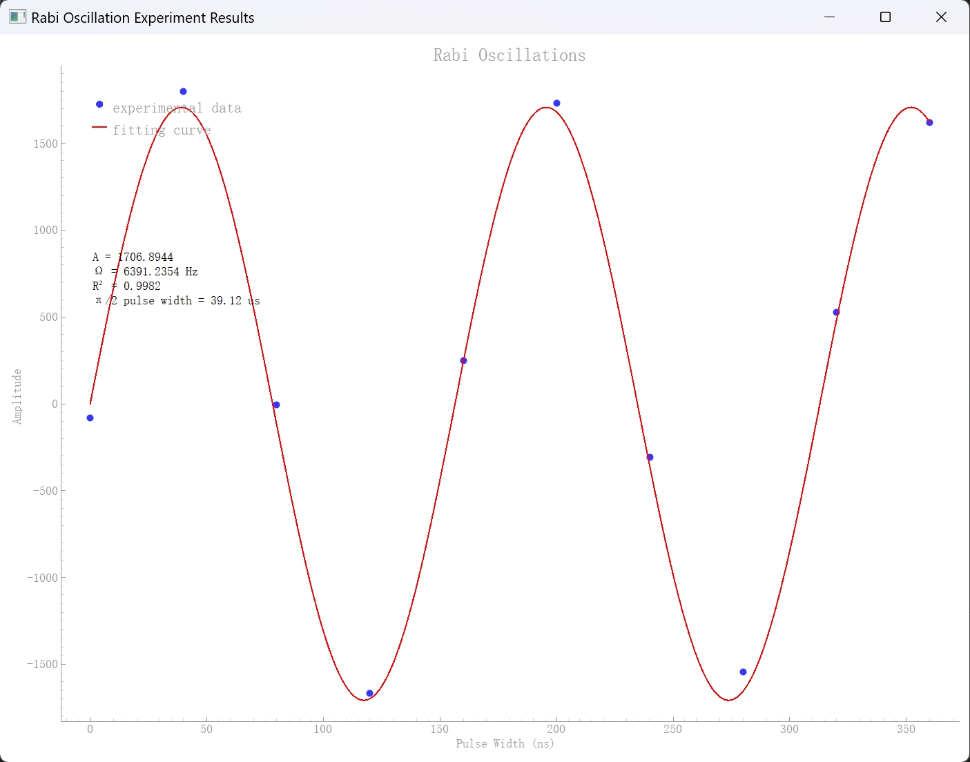
Rabi oscillation experiment
Measure Rabi oscillations at different pulse widths to determine π/2 and π pulse widths:
import time
import numpy as np
from scipy.optimize import curve_fit
import matplotlib.pyplot as plt
from spinqlablink import SpinQLabLink, ExperimentType, Pulse

def rabi_oscillation_experiment():
    """Rabi Oscillation Experiment - Pulse Width Scanning"""
    spinqlablink = SpinQLabLink("192.168.9.121", 8181, "username", "password")
    spinqlablink.connect()
    spinqlablink.wait_for_login()

    # Pulse width range
    width_list = [i * 40 for i in range(10)]  # 0, 40, 80, ..., 360 μs
    intensities = []

    try:
        for width in width_list:
            print(f"Testing pulse width: {width} μs")

            # Register experiment
            _, exp_para = spinqlablink.register_experiment(ExperimentType.RABI_OSCILLATIONS)

            # Set parameters
            exp_para.freq_h = 37.852105
            exp_para.freq_p = 15.322872
            exp_para.makePps = True
            exp_para.samplePath = 0
            exp_para.custom_freq = False
            exp_para.pulses = [Pulse(path=0, width=width, amplitude=100, phase=90, detuning=0)]

            # Run experiment
            spinqlablink.run_experiment()
            spinqlablink.wait_for_experiment_completion()

            # Get results
            result = spinqlablink.get_experiment_result()
            signal_data = result["result"]["real"]

            # Calculate signal intensity (FFT peak)
            if signal_data is not None:
                if isinstance(signal_data, (int, float)):
                    signal_array = np.array([signal_data])
                elif isinstance(signal_data, (list, tuple, np.ndarray)):
                    signal_array = np.array([point[1] for point in signal_data if isinstance(point, (list, tuple, np.ndarray))])
                else:
                    signal_array = np.array([])
                if len(signal_array) > 0:
                    intensity = np.max(np.abs(np.fft.fft(signal_array)))
                else:
                    intensity = 0
                intensities.append(intensity)
            else:
                intensities.append(0)

            spinqlablink.deregister_experiment()
            time.sleep(2)  # Wait for system stabilization

        # Fit Rabi oscillation curve
        def rabi_function(x, A, B, freq, phase):
            return A * np.cos(2 * np.pi * freq * x + phase) + B

        try:
            popt, _ = curve_fit(rabi_function, width_list, intensities)
            pi_pulse_width = np.pi / (2 * np.pi * popt[2])
            print(f"Estimated π pulse width: {pi_pulse_width:.1f} μs")

            # Plot results
            plt.figure(figsize=(10, 6))
            plt.plot(width_list, intensities, 'bo-', label='Experimental data')
            x_fit = np.linspace(min(width_list), max(width_list), 100)
            y_fit = rabi_function(x_fit, *popt)
            plt.plot(x_fit, y_fit, 'r-', label='Fitted curve')
            plt.xlabel('Pulse width (μs)')
            plt.ylabel('Signal intensity')
            plt.title('Rabi Oscillation')
            plt.legend()
            plt.grid(True)
            plt.show()

        except Exception as e:
            print(f"Fitting failed: {e}")

    finally:
        spinqlablink.disconnect()

if __name__ == "__main__":
    rabi_oscillation_experiment()
Experimental Parameters Analysis
ExperimentType: Select RABI_OSCILLATIONS for experimental type (see:class:spinqlablink.ExperimentType class for details)
Pulse: Define the pulse sequence and set the path, width, amplitude, phase and frequency offset of the pulse (see:class:spinqlablink.Pulse class for details)
freq_h: Hydrogen resonance frequency (hz) [0- 100M]
freq_p: Phosphorus resonance frequency (hz) [0- 100M]
makePps: Whether to use PPS pulse sequences
samplePath: Sampling path, 0= hydrogen channel, 1= phosphorus channel [0-1]
custom_freq: Whether to use custom frequency [True,False]
Code flow analysis
The code flow of the Rabi Oscillation experiment can be divided into the following key steps:
** Initialize connection **:
Create a SpinQLabLink object and connect it to a quantum computing device
Verify login status and ensure successful connection
** Experimental parameter settings **:
Register Rabbi Oscillation Experiments (RABI_OSCILLATIONS)
Set experimental parameters, including resonance frequency, sampling path, etc.
Define a list of pulse widths for observing oscillation effects at different widths
** Experimental execution cycle **:
Iterates for each pulse width
Set the corresponding pulse parameters for each iteration
Run the experiment and wait for completion
Collect experimental results and extract signal strength data
Log out experiments between iterations and wait for the system to stabilize
** Data analysis and visualization **:
Fitting Rabi oscillation curve using nonlinear least squares method
Calculate π pulse width from fitting parameters
Plot experimental data points and fitted curves
Display results chart
** Resource release **:
Disconnect the connection from the device after the experiment is completed
This experiment demonstrates the Rabi oscillation phenomenon of qubits under the action of radio frequency pulses by observing the changes in signal strength under different pulse widths. This is the basis of quantum control and an important method for determining the π pulse width (used for qubit flipping).
Analysis of experimental results
{
    "result":{
        "graph":[
            { # step 0
                "fidRe": [[x,y],...],
                "fidIm":[[x,y],...],
                "fftRe":[[x,y],...],
                "fftIm":[[x,y],...],
                "lorenz":[[x,y],...],
                "fftMod":[[x,y],...]
            }
        ],
        "width": 80.0, # Pulse Width
        "real": 0.85 # Real part of signal strength
    }
}
graph: Chart data, including real and imaginary parts, the graph contains 1 step
width: Pulse width
real: real part of signal strength
qubit experiment
Observe the physical properties of qubits
from spinqlablink import SpinQLabLink, ExperimentType, Pulse
from spinqlablink import print_graph

def main():
    # Create connection
    spinqlablink = SpinQLabLink("192.168.15.4", 8181, "anyword", "anyword")
    spinqlablink.connect()

    if not spinqlablink.wait_for_login():
        print("Login failed")
        return

    # Register Quantum Bit experiment
    # This experiment demonstrates the basic operations and measurements of a single qubit
    # In NMR systems, nuclear spins serve as qubits with two energy states (|0⟩ and |1⟩)
    _, exp_qubit_para = spinqlablink.register_experiment(ExperimentType.QUANTUM_BIT)

    # Set experiment parameters
    # Channel selection
    exp_qubit_para.samplePath = 0  # Sampling path: 0=Hydrogen channel, 1=Phosphorus channel
                                # Hydrogen nuclei are commonly used as qubits in NMR quantum computing

    # Define the pulse sequence for qubit manipulation
    # This example uses a π/2 pulse (90° rotation) which creates a superposition state
    # Parameters:
    # - path: 0 for hydrogen channel
    # - width: 40 microseconds pulse duration
    # - amplitude: 100% of maximum amplitude
    # - phase: 90 degrees phase angle (creates rotation around Y-axis)
    # - detuning: 0 Hz frequency offset from resonance
    exp_qubit_para.pulses = [Pulse(path=0,width=40, amplitude=100, phase=90, detuning=0)]

    # Run the experiment
    spinqlablink.run_experiment()
    print("Waiting for experiment completion")
    spinqlablink.wait_for_experiment_completion()

    # Get the results
    exp_info = spinqlablink.get_experiment_result()

    # Clean up and disconnect
    spinqlablink.deregister_experiment()
    spinqlablink.disconnect()

    # Display the results
    # The results should show the quantum state of the qubit after manipulation
    if "result" in exp_info:
        exp_result = exp_info["result"]
        for key, value in exp_result.items():
            if key != "graph":
                print(f"{key}: {value}")

        print_graph(exp_info["result"])
    else:
        print("Experiment failed")

if __name__ == "__main__":
    main()
Experimental Parameters Analysis
ExperimentType: Select QUANTUM_BIT for experimental type (see:class:spinqlablink.ExperimentType class for details)
Pulse: Define the pulse sequence and set the path, width, amplitude, phase and frequency offset of the pulse (see:class:spinqlablink.Pulse class for details)
samplePath: Sampling path, 0= hydrogen channel, 1= phosphorus channel [0-1]
pulses: List of pulse sequences, containing a series of Pulse objects
Analysis of experimental results
{
    "result":{
        "graph":[
            { # step 0
                "fidRe": [[x,y],...],
                "fidIm":[[x,y],...],
                "fftRe":[[x,y],...],
                "fftIm":[[x,y],...],
                "lorenz":[[x,y],...],
                "fftMod":[[x,y],...]
            }
        ],
        "coordinate": {  # The coordinates of a qubit on the Bloch sphere
            "x": [0, 1],
            "y": [0, 1],
            "z": [0, 1]
        },
        "matrix": {  # The density matrix of a quantum state, including its real and imaginary parts
            "real": [[1, 0], [0, 1]],
            "imag": [[0, 0], [0, 0]]
        },
        "probability": [0.5, 0.5]  # Probability distribution of measurement results
    }
}
graph: Chart data, including real and imaginary parts, the graph contains 2 steps
coordinate: The coordinates of the qubit on the Bloch sphere
matrix: The density matrix of the quantum state, including the real and imaginary parts
probability: probability distribution of measurement results
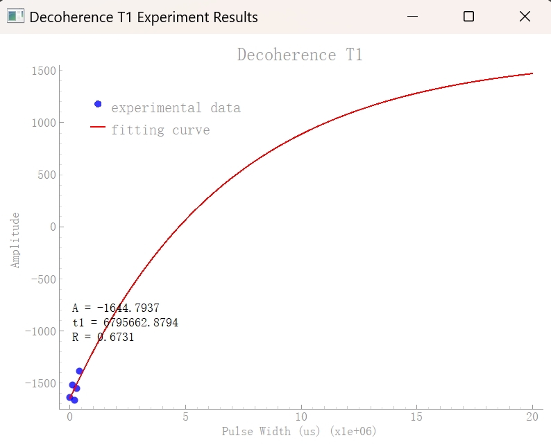
Quantum decoherence T1 experiment
Observation of quantum decoherence phenomenon T1
from spinqlablink import SpinQLabLink, ExperimentType, Pulse

# Drawing charts
import pyqtgraph as pg
from pyqtgraph.Qt import QtWidgets
import numpy as np
from scipy.optimize import curve_fit

def main():
    # Create connection
    spinqlablink = SpinQLabLink("192.168.15.4", 8181, "anyword", "anyword")
    spinqlablink.connect()

    if not spinqlablink.wait_for_login():
        print("Login failed")
        return

    width_real_map = {}
    width_list = []

    for i in range(5):
        width_list.append(i * 100000)

    for width in width_list:
        _, exp_decot1_para = spinqlablink.register_experiment(ExperimentType.QUANTUM_DECOHERENCE_T1)

        # Set other parameters
        exp_decot1_para.samplePath = 0  # Sampling path: 0=Hydrogen channel, 1=Phosphorus channel

        exp_decot1_para.pulses = [Pulse(path=0,width=80, amplitude=100, phase=90, detuning=0)
                                ,Pulse(path=0,width=width, amplitude=0, phase=0, detuning=0)]

        spinqlablink.run_experiment()
        print("Waiting for experiment completion")
        spinqlablink.wait_for_experiment_completion()

        exp_info = spinqlablink.get_experiment_result()

        width_real_map[width] = exp_info["result"]["real"]

        spinqlablink.deregister_experiment()

    spinqlablink.disconnect()

    print("width_real_map: ", width_real_map)
    # Convert data to format suitable for fitting
    x_data = list(width_real_map.keys())
    y_data = list(width_real_map.values())

    # Plot experiment results and fitting curve
    app = QtWidgets.QApplication([])
    win = pg.GraphicsLayoutWidget(show=True, title="Rabi Oscillation Experiment Results")
    win.resize(800, 600)

    # Set background to white
    win.setBackground('w')

    # Add plot area
    plot = win.addPlot(title="Decoherence T1")
    plot.setLabel('left', 'Amplitude')
    plot.setLabel('bottom', 'Pulse Width (us)')

    # Execute fitting and display results
    fit_results = fit_decot1_oscillations(x_data, y_data, plot)

    # Start Qt event loop
    app.exec_()

def fit_decot1_oscillations(x_data, y_data, plot):
    """
    Fit T1 relaxation data with an exponential decay model and display the results.

    T1 relaxation (longitudinal/amplitude relaxation) follows the model:
    A + (|A| - A) * (1 - exp(-t/T1))

    where:
    - A is the equilibrium amplitude
    - T1 is the relaxation time constant
    - t is the delay time

    Parameters:
        x_data: List of delay times (in microseconds)
        y_data: Corresponding experimental signal amplitudes
        plot: pyqtgraph Plot object to display the results

    Returns:
        Dictionary containing fitting parameters: A (equilibrium amplitude),
        T1 (relaxation time), and R (correlation coefficient)
    """
    # Draw experimental data points
    scatter = pg.ScatterPlotItem(x=x_data, y=y_data, pen=None, brush=pg.mkBrush(0, 0, 255, 200), size=10)
    plot.addItem(scatter)

    # Prepare fitting parameters
    min_sig = min(y_data)

    # T1 relaxation model: equilibrium + (max_change) * (1 - exp(-t/T1))
    # This models how the system returns to equilibrium after excitation
    def t1_model(x, A, t1):
        return A + (np.abs(A) - A) * (1 - np.exp(-x / t1));

    # Initial parameter guesses: equilibrium amplitude and approximate T1 time
    p0 = [min_sig, 5000000]

    # Execute fitting
    try:
        popt, pcov = curve_fit(t1_model, x_data, y_data, p0=p0)

        # Get fitting parameters
        A_fit, t1_fit = popt

        # Calculate fitting quality R² (coefficient of determination)
        # R² = 1 - (residual sum of squares / total sum of squares)
        residuals = y_data - t1_model(np.array(x_data), *popt)
        ss_res = np.sum(residuals**2)
        ss_tot = np.sum((y_data - np.mean(y_data))**2)
        r = np.sqrt(1 - (ss_res / ss_tot))

        # Generate fitting curve with higher resolution for smooth display
        x_fit = np.linspace(0, 20000000, 5000)
        y_fit = t1_model(x_fit, *popt)

        # Draw fitting curve
        fit_curve = pg.PlotCurveItem(x=x_fit, y=y_fit, pen=pg.mkPen('r', width=2))
        plot.addItem(fit_curve)

        # Add legend
        legend = plot.addLegend()
        legend.addItem(scatter, 'experimental data')
        legend.addItem(fit_curve, 'fitting curve')

        # Display fitting parameters
        text = pg.TextItem(text=f"A = {A_fit:.4f}\nt1 = {t1_fit:.4f}\nR = {r:.4f}",
                        color=(0, 0, 0), anchor=(0, 0))
        text.setPos(min(x_data), max(y_data) * 0.5)
        plot.addItem(text)

        print("fitting parameters:")
        print(f"A = {A_fit:.4f}")
        print(f"t1 = {t1_fit:.4f}")
        print(f"fitting quality R = {r:.4f}")

        return {
            "A": A_fit,
            "t1": t1_fit,
            "r": r
        }

    except Exception as e:
        print(f"fitting error: {e}")
        return None


if __name__ == "__main__":
    main()
Experimental Parameters Analysis
ExperimentType: Select QUANTUM_DECOHERENCE_T1 for experimental type (see:class:spinqlablink.ExperimentType class for details)
Pulse: Define the pulse sequence and set the path, width, amplitude, phase and frequency offset of the pulse (see:class:spinqlablink.Pulse class for details)
samplePath: Sampling path, 0= hydrogen channel, 1= phosphorus channel [0-1]
pulses: List of pulse sequences, containing a series of Pulse objects, usually containing two pulses: -First pulse: π/2 pulse, used to excite the qubit-Second pulse: delayed pulse, width change used to measure T1 relaxation time
Code flow analysis
The code flow of the quantum decoherence T1 experiment can be divided into the following key steps:
** Initialize connection **:
Create a SpinQLabLink object and connect it to a quantum computing device
Verify login status and ensure successful connection
** Preparation of experimental parameters **:
Create a data structure to store measurement results with different latency times
Define a list of delay times for observing the relaxation process of qubits
** Experimental execution cycle **:
Iterates for each delay time
Register the Quantum Decoherence T1 Experiment (QUANTUM_DECOHERENCE_T1)
Set experimental parameters, including sampling path and pulse sequence
A pulse sequence usually consists of two pulses:
The first pulse: π/2 pulse (90°), which transfers the qubit from| Excitation of 0 state to superposition state
Second pulse: delayed pulse, with varying width used to measure quantum states after different waiting times
Run the experiment and wait for completion
Collect experimental results and extract signal strength data
Cancel experiments between iterations
** Data analysis and fitting **:
Fit the T1 relaxation curve using an exponential decay model: f(t) = A * exp(-t/T1) + C
Extraction of T1 time constant from fitting parameters
Calculate the fitting quality (R value) to evaluate the fitting accuracy
** Results visualization **:
Plot experimental data points and fitted curves
Display fitting parameters, including amplitude A, T1 time, and fit quality R
Add legend and parameter text to the chart
** Resource release **:
Disconnect the connection from the device after the experiment is completed
This experiment measured the longitudinal relaxation time (T1) of the qubit by observing the process of returning the qubit from the excited state to the ground state. This is an important parameter for evaluating the quality of the qubit and represents the time scale on which the qubit can retain energy.
Analysis of experimental results
{
    "result":{
        "graph":[
            { # step 0
                "fidRe": [[x,y],...],
                "fidIm":[[x,y],...],
                "fftRe":[[x,y],...],
                "fftIm":[[x,y],...],
                "lorenz":[[x,y],...],
                "fftMod":[[x,y],...]
            }
        ],
        "width": 100000,  # Delay pulse width
        "real": 0.75,  # Real part of signal strength
        "coordinate": {  # The coordinates of a qubit on the Bloch sphere
            "x": [0, 1],
            "y": [0, 1],
            "z": [0, 1]
        },
        "matrix": {  # The density matrix of a quantum state, including its real and imaginary parts
            "real": [[1, 0], [0, 1]],
            "imag": [[0, 0], [0, 0]]
        },
        "probability": [0.5, 0.5]  # Probability distribution of measurement results
    }
}
graph: Chart data, including real and imaginary parts, the graph contains 2 steps
width: Delay pulse width
real: real part of signal strength
coordinate: The coordinates of the qubit on the Bloch sphere
matrix: The density matrix of the quantum state, including the real and imaginary parts
probability: probability distribution of measurement results
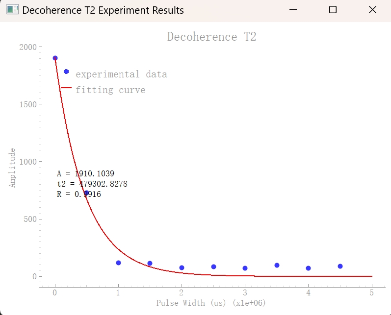
Quantum decoherence T2 experiment
Observation of quantum decoherence phenomenon T2
from spinqlablink import SpinQLabLink, ExperimentType, Pulse

# Drawing charts
import pyqtgraph as pg
from pyqtgraph.Qt import QtWidgets
import numpy as np
from scipy.optimize import curve_fit

def main():
    # Create connection
    spinqlablink = SpinQLabLink("192.168.15.4", 8181, "anyword", "anyword")
    spinqlablink.connect()

    if not spinqlablink.wait_for_login():
        print("Login failed")
        return

    width_mod_map = {}
    width_list = []

    for i in range(10):
        width_list.append(i * 500000)

    for width in width_list:
        _, exp_decot2_para = spinqlablink.register_experiment(ExperimentType.QUANTUM_DECOHERENCE_T2)

        # Set other parameters
        exp_decot2_para.samplePath = 0  # Sampling path: 0=Hydrogen channel, 1=Phosphorus channel

        exp_decot2_para.pulses = [Pulse(path=0,width=40, amplitude=100, phase=90, detuning=0)
                                ,Pulse(path=0,width=width/2, amplitude=0, phase=0, detuning=0)
                                ,Pulse(path=0,width=80, amplitude=100, phase=90, detuning=0)
                                ,Pulse(path=0,width=width/2, amplitude=0, phase=0, detuning=0)]

        spinqlablink.run_experiment()
        print("Waiting for experiment completion")
        spinqlablink.wait_for_experiment_completion()

        exp_info = spinqlablink.get_experiment_result()

        width_mod_map[width] = exp_info["result"]["mod"]

        spinqlablink.deregister_experiment()

    spinqlablink.disconnect()

    print("width_mod_map: ", width_mod_map)
    # Convert data to format suitable for fitting
    x_data = list(width_mod_map.keys())
    y_data = list(width_mod_map.values())

    # Plot experiment results and fitting curve
    app = QtWidgets.QApplication([])
    win = pg.GraphicsLayoutWidget(show=True, title="Decoherence T2 Experiment Results")
    win.resize(800, 600)

    # Set background to white
    win.setBackground('w')

    # Add plot area
    plot = win.addPlot(title="Decoherence T2")
    plot.setLabel('left', 'Amplitude')
    plot.setLabel('bottom', 'Pulse Width (us)')

    # Execute fitting and display results
    fit_results = fit_decot2_oscillations(x_data, y_data, plot)

    # Start Qt event loop
    app.exec_()

def fit_decot2_oscillations(x_data, y_data, plot):
    """
    Fit Decoherence t2 oscillation data with a sine function and display the results on the specified plot

    Parameters:
        x_data: List of pulse widths
        y_data: Corresponding experimental data
        plot: pyqtgraph Plot object to display the results

    Returns:
        Fitting parameters and results
    """
    # Draw experimental data points
    scatter = pg.ScatterPlotItem(x=x_data, y=y_data, pen=None, brush=pg.mkBrush(0, 0, 255, 200), size=10)
    plot.addItem(scatter)

    # Prepare fitting parameters
    max_sig = max(y_data)

    # Decoherence T2 fitting function A * exp(- x / B)
    def t2_model(x, A, t2):
        return abs(A) * np.exp(- x / t2);

    p0 = [max_sig, 500000]

    # Execute fitting
    try:
        popt, pcov = curve_fit(t2_model, x_data, y_data, p0=p0)

        # Get fitting parameters
        A_fit, t2_fit = popt

        # Calculate fitting quality R²
        residuals = y_data - t2_model(np.array(x_data), *popt)
        ss_res = np.sum(residuals**2)
        ss_tot = np.sum((y_data - np.mean(y_data))**2)
        r = np.sqrt(1 - (ss_res / ss_tot))

        # Generate fitting curve
        x_fit = np.linspace(0, 5000000, 1000)
        y_fit = t2_model(x_fit, *popt)

        # Draw fitting curve
        fit_curve = pg.PlotCurveItem(x=x_fit, y=y_fit, pen=pg.mkPen('r', width=2))
        plot.addItem(fit_curve)

        # Add legend
        legend = plot.addLegend()
        legend.addItem(scatter, 'experimental data')
        legend.addItem(fit_curve, 'fitting curve')

        # Display fitting parameters
        text = pg.TextItem(text=f"A = {A_fit:.4f}\nt2 = {t2_fit:.4f}\nR = {r:.4f}",
                        color=(0, 0, 0), anchor=(0, 0))
        text.setPos(min(x_data), max(y_data) * 0.5)
        plot.addItem(text)

        print("fitting parameters:")
        print(f"A = {A_fit:.4f}")
        print(f"t2 = {t2_fit:.4f}")
        print(f"fitting quality R = {r:.4f}")

        return {
            "A": A_fit,
            "t2": t2_fit,
            "r": r
        }

    except Exception as e:
        print(f"fitting error: {e}")
        return None


if __name__ == "__main__":
    main()
Experimental Parameters Analysis
ExperimentType: Select QUANTUM_DECOHERENCE_T2 for experimental type (see:class:spinqlablink.ExperimentType class for details)
Pulse: Define the pulse sequence and set the path, width, amplitude, phase and frequency offset of the pulse (see:class:spinqlablink.Pulse class for details)
samplePath: Sampling path, 0= hydrogen channel, 1= phosphorus channel [0-1]
pulses: List of pulse sequences, containing a series of Pulse objects, usually containing four pulses: -First pulse: π/2 pulse, used to excite the qubit-Second pulse: delayed pulse, width change used to measure T2 relaxation time-Third pulse: π pulse, used to echo-Fourth pulse: delayed pulse, width change used to measure T2 relaxation time
Code flow analysis
The code flow of the quantum decoherence T2 experiment can be divided into the following key steps:
** Initialize connection **:
Create a SpinQLabLink object and connect it to a quantum computing device
Verify login status and ensure successful connection
** Preparation of experimental parameters **:
Create a data structure to store measurement results with different latency times
Define a list of delay times for observing the decay of coherence of qubits over time
** Experimental execution cycle **:
Iterates for each delay time
Register the Quantum Decoherence T2 Experiment (QUANTUM_DECOHERENCE_T2)
Set experimental parameters, including sampling path and pulse sequence
The pulse sequence usually contains four pulses:
The first pulse: π/2 pulse (90°), which transfers the qubit from| The 0 state is excited to the equatorial plane
Second pulse: delayed pulse, width variation used to measure free evolution time
The third pulse: π pulse (180°), used for echo formation, canceling static field inhomogeneities
Fourth pulse: Delayed pulse, same width as the second pulse, used for echo formation
Run the experiment and wait for completion
Collect experimental results and extract signal strength data
Cancel experiments between iterations
** Data analysis and fitting **:
Fit T2 relaxation curve using exponential decay model: f(t) = A * exp(-t/T2)
Extraction of T2 time constant from fitting parameters
Calculate the fitting quality (R value) to evaluate the fitting accuracy
** Results visualization **:
Plot experimental data points and fitted curves
Displays fit parameters, including amplitude A, T2 time, and fit quality R
Add legend and parameter text to the chart
** Resource release **:
Disconnect the connection from the device after the experiment is completed
This experiment measures the lateral relaxation time (T2) of the qubit by observing the decay of the coherence of the qubit over time. This is another important parameter for evaluating the quality of the qubit and represents the time scale at which the qubit can maintain a coherent superposition state. T2 time is usually shorter than T1 time because coherence is more sensitive to environmental noise.
Analysis of experimental results
{
    "result":{
        "graph":[
            { # step 0
                "fidRe": [[x,y],...],
                "fidIm":[[x,y],...],
                "fftRe":[[x,y],...],
                "fftIm":[[x,y],...],
                "lorenz":[[x,y],...],
                "fftMod":[[x,y],...]
            }
        ],
        "width": 500000,  # Delay pulse width
        "mod": 0.65,  # Signal Strength Magnitude
        "coordinate": {  # The coordinates of a qubit on the Bloch sphere
            "x": [0, 1],
            "y": [0, 1],
            "z": [0, 1]
        },
        "matrix": {  # The density matrix of a quantum state, including its real and imaginary parts
            "real": [[1, 0], [0, 1]],
            "imag": [[0, 0], [0, 0]]
        },
        "probability": [0.5, 0.5]  # Probability distribution of measurement results
    }
}
graph: Chart data, including real and imaginary parts, the graph contains 2 steps
width: Delay pulse width
mod: Signal strength modulus
coordinate: The coordinates of the qubit on the Bloch sphere
matrix: The density matrix of the quantum state, including the real and imaginary parts
probability: probability distribution of measurement results
quantum control experiment
Using radio frequency fields to regulate the state of qubits
from spinqlablink import SpinQLabLink, ExperimentType, Pulse
from spinqlablink import print_graph

def main():
    # Create connection
    spinqlablink = SpinQLabLink("192.168.15.4", 8181, "anyword", "anyword")
    spinqlablink.connect()

    if not spinqlablink.wait_for_login():
        print("Login failed")
        return

    _, exp_qcontrol_para = spinqlablink.register_experiment(ExperimentType.QUANTUM_CONTROL)

    # Set other parameters
    exp_qcontrol_para.samplePath = -1  # Sampling path: 0=Hydrogen channel, 1=Phosphorus channel

    exp_qcontrol_para.pulses = [Pulse(path=0,width=40, amplitude=100, phase=90, detuning=0),
                                Pulse(path=1,width=40, amplitude=100, phase=90, detuning=0)]

    spinqlablink.run_experiment()
    print("Waiting for experiment completion")
    spinqlablink.wait_for_experiment_completion()

    exp_info = spinqlablink.get_experiment_result()

    spinqlablink.deregister_experiment()

    spinqlablink.disconnect()

    if "result" in exp_info:
        exp_result = exp_info["result"]
        for key, value in exp_result.items():
            if key != "graph":
                print(f"{key}: {value}")

        print_graph(exp_info["result"])
    else:
        print("Experiment failed")

if __name__ == "__main__":
    main()
Experimental Parameters Analysis
ExperimentType: Select QUANTUM_CONTROL for experimental type (see:class:spinqlablink.ExperimentType class for details)
Pulse: Define the pulse sequence and set the path, width, amplitude, phase and frequency offset of the pulse (see:class:spinqlablink.Pulse class for details)
samplePath: Sampling path,-1= all channels, 0= hydrogen channel, 1= phosphorus channel [-1,0,1]
pulses: List of pulse sequences, containing a series of Pulse objects, which contain two pulses: -First pulse: π/2 pulse acting on the hydrogen channel (path=0)-Second pulse: π/2 pulse acting on the phosphorus channel (path=1)
Analysis of experimental results
{
    "result":{
        "graph":[
            { # step 0
                "fidRe": [[x,y],...],
                "fidIm":[[x,y],...],
                "fftRe":[[x,y],...],
                "fftIm":[[x,y],...],
                "lorenz":[[x,y],...],
                "fftMod":[[x,y],...]
            },
            { # step 1
                "fidRe": [[x,y],...],
                "fidIm":[[x,y],...],
                "fftRe":[[x,y],...],
                "fftIm":[[x,y],...],
                "lorenz":[[x,y],...],
                "fftMod":[[x,y],...]
            }
        ],
        "coordinate": {  # The coordinates of a qubit on the Bloch sphere
            "x": [0, 1],
            "y": [0, 1],
            "z": [0, 1]
        },
        "matrix": {  # The density matrix of a two-qubit system, including the real and imaginary parts
            "real": [[1, 0, 0, 0], [0, 1, 0, 0], [0, 0, 1, 0], [0, 0, 0, 1]],
            "imag": [[0, 0, 0, 0], [0, 0, 0, 0], [0, 0, 0, 0], [0, 0, 0, 0]]
        },
        "probability": [0.25, 0.25, 0.25, 0.25]  # Probability distribution of measurement results
    }
}
graph: Chart data, the graph contains 2/6 steps
coordinate: The coordinates of the qubit on the Bloch sphere
matrix: The density matrix of two qubit systems, including real and imaginary parts
probability: probability distribution of measurement results
Quantum system initialization experiment
Implement the initialization process of quantum systems
from spinqlablink import SpinQLabLink, ExperimentType, Pulse
from spinqlablink import print_graph

def main():
    # Create connection
    spinqlablink = SpinQLabLink("192.168.15.4", 8181, "anyword", "anyword")
    spinqlablink.connect()

    if not spinqlablink.wait_for_login():
        print("Login failed")
        return

    _, exp_sysinit_para = spinqlablink.register_experiment(ExperimentType.QUANTUM_SYSTEM_INITIALIZATION)

    # Set other parameters
    exp_sysinit_para.repeat = 9

    exp_sysinit_para.pulses = [Pulse(path=0,phase=90,amplitude=100,width=40),
                                Pulse(path=0,phase=0,amplitude=0,width=718),
                                Pulse(path=0,phase=0,amplitude=100,width=40),
                                Pulse(path=0,phase=0,amplitude=0,width=718),
                                Pulse(path=0,phase=0,amplitude=0,width=40),
                                Pulse(path=0,phase=0,amplitude=0,width=500000),
                                Pulse(path=1,phase=0,amplitude=0,width=40),
                                Pulse(path=1,phase=0,amplitude=0,width=718),
                                Pulse(path=1,phase=90,amplitude=100,width=40),
                                Pulse(path=1,phase=0,amplitude=0,width=718),
                                Pulse(path=1,phase=0,amplitude=100,width=40),
                                Pulse(path=1,phase=0,amplitude=0,width=500000)]

    spinqlablink.run_experiment()
    print("Waiting for experiment completion")
    spinqlablink.wait_for_experiment_completion()

    exp_info = spinqlablink.get_experiment_result()

    spinqlablink.deregister_experiment()

    spinqlablink.disconnect()

    if "result" in exp_info:
        exp_result = exp_info["result"]
        for key, value in exp_result.items():
            if key != "graph":
                print(f"{key}: {value}")

        print_graph(exp_info["result"])
    else:
        print("Experiment failed")

if __name__ == "__main__":
    main()
Experimental Parameters Analysis
ExperimentType: Select QUANTUM_SYSTEM_INITIALIZATION for experimental type (see:class:spinqlablink.ExperimentType class for details)
Pulse: Define the pulse sequence and set the path, width, amplitude, phase and frequency offset of the pulse (see:class:spinqlablink.Pulse class for details)
Repeat: The number of repeats is used to enhance signal strength, usually set to 9 times
pulses: Pulse sequence list, containing a series of Pulse objects, which contains 12 pulses: -First 6 pulses: Pulse sequence acting on the hydrogen channel (path=0), used to initialize hydrogen nuclear spin-Last 6 pulses: Pulse sequence acting on the phosphorus channel (path=1), used to initialize phosphorus nuclear spin
Analysis of experimental results
{
    "result":{
        "graph":[
            { # step 0
                "fidRe": [[x,y],...],
                "fidIm":[[x,y],...],
                "fftRe":[[x,y],...],
                "fftIm":[[x,y],...],
                "lorenz":[[x,y],...],
                "fftMod":[[x,y],...]
            },
            { # step 1
                "fidRe": [[x,y],...],
                "fidIm":[[x,y],...],
                "fftRe":[[x,y],...],
                "fftIm":[[x,y],...],
                "lorenz":[[x,y],...],
                "fftMod":[[x,y],...]
            }
        ],
        "Hlamda": 8349439,  # Lambda parameter of the hydrogen nucleus
        "Plamda": 2714902,  # Lambda parameter of the hydrogen nucleus
        "coordinate": {  # The coordinates of the qubit on the Bloch sphere, initialized to the |00⟩ state
            "x": [0, 0],
            "y": [0, 0],
            "z": [1, 1]
        },
        "matrix": {  # The density matrix of a two-qubit system, initialized in the |00⟩ state
            "real": [[1, 0, 0, 0], [0, 0, 0, 0], [0, 0, 0, 0], [0, 0, 0, 0]],
            "imag": [[0, 0, 0, 0], [0, 0, 0, 0], [0, 0, 0, 0], [0, 0, 0, 0]]
        },
        "probability": [1, 0, 0, 0]  # The probability distribution of measurement results, initialized with the probability of the |00⟩ state being 1
    }
}
graph: Chart data, the graph contains 6 steps
Hlamda: Lambda parameter of the hydrogen core, used for custom PPS settings in subsequent experiments
Plamda: Lambda parameter of the phosphorus core, used for custom PPS settings in subsequent experiments
coordinate: The coordinates of the qubit on the Bloch sphere, initialized to| 00 丨 state
matrix: density matrix of a two-qubit system, initialized to| 00 丨 state
probability: The probability distribution of the measurement result, initialized to| The probability of the 00 state is 1
Quantum logic gates and quantum circuits
Build quantum gates and quantum circuits based on control operations
from spinqlablink import SpinQLabLink, ExperimentType, Pulse, Gate, CustomGate, Circuit
from spinqlablink import print_graph

def main():
    # Create connection
    spinqlablink = SpinQLabLink("192.168.15.4", 8181, "anyword", "anyword")
    spinqlablink.connect()

    if not spinqlablink.wait_for_login():
        print("Login failed")
        return

    _, exp_gates_and_circuit_para = spinqlablink.register_experiment(ExperimentType.QUANTUM_GATES_AND_CIRCUIT)

    # Configuration flags
    using_pulse = False      # True: use direct pulse sequence, False: use quantum gates
    using_custom_gate = False  # True: use custom-defined gates, False: use built-in gates
    using_custom_pps = False   # True: use custom Pseudo-Pure State initialization, False: use default PPS

    # Custom PPS (Pseudo-Pure State) initialization sequence
    # This JSON defines pulse sequences for both channels (hydrogen and phosphorus)
    pps_json = '{"pulse":{"channel1_pulse":[{"amplitude":100.0,"detuning":0.0,"phase":90.0,"width":40.0},{"amplitude":0,"detuning":0.0,"phase":0.0,"width":718.0},{"amplitude":0,"detuning":0.0,"phase":0.0,"width":40.0},{"amplitude":0,"detuning":0.0,"phase":0.0,"width":718.0},{"amplitude":100,"detuning":0.0,"phase":0.0,"width":40.0},{"amplitude":0,"detuning":0.0,"phase":0.0,"width":500000.0}],"channel2_pulse":[{"amplitude":0,"detuning":0.0,"phase":0.0,"width":40.0},{"amplitude":0,"detuning":0.0,"phase":0.0,"width":718.0},{"amplitude":100.0,"detuning":0.0,"phase":90.0,"width":40.0},{"amplitude":0,"detuning":0.0,"phase":0.0,"width":718.0},{"amplitude":100.0,"detuning":0.0,"phase":0.0,"width":40.0},{"amplitude":0,"detuning":0.0,"phase":0.0,"width":500000.0}]}}'

    # System parameters from system initialization experiment
    Hlamda = 8349439  # Hydrogen lambda parameter (obtained from system initialization)
    Plamda = 2714902  # Phosphorus lambda parameter (obtained from system initialization)

    # Set experiment parameters
    exp_gates_and_circuit_para.samplePath = -1 # -1 for all channels, 0 for hydrogen channel, 1 for phosphorus channel
    exp_gates_and_circuit_para.using_pulse = using_pulse # True for using pulse, False for using gate

    if not using_pulse:
        exp_gates_and_circuit_para.using_custom_gate = using_custom_gate # True for using custom gate, False for using default gate
        exp_gates_and_circuit_para.using_custom_pps = using_custom_pps # True for using custom pps, False for using default pps

        # Configure custom PPS parameters if enabled
        if using_custom_pps:
            exp_gates_and_circuit_para.pps_repeat = 9  # Number of times to repeat the PPS sequence
            exp_gates_and_circuit_para.pps_json = pps_json  # Custom PPS pulse sequence
            exp_gates_and_circuit_para.Hlamda = Hlamda  # Hydrogen lambda parameter for PPS
            exp_gates_and_circuit_para.Plamda = Plamda  # Phosphorus lambda parameter for PPS

        # Create a 2-qubit quantum circuit
        circuit = Circuit(2)

        if using_custom_gate: # using custom gate
            # Example of custom gate definition using JSON (commented out)
            # H0_file_json = '{"pulse":{"channel1_pulse":[{"amplitude":100.0,"detuning":0.0,"phase":90.0,"width":40.0}],"channel2_pulse":[{"amplitude":0.0,"detuning":0.0,"phase":0.0,"width":40.0}]}}'
            # H1_file_json = '{"pulse":{"channel1_pulse":[{"amplitude":0.0,"detuning":0.0,"phase":0.0,"width":40.0}],"channel2_pulse":[{"amplitude":100.0,"detuning":0.0,"phase":90.0,"width":40.0}]}}'
            # circuit << CustomGate(type='H',customType='H_custom_gate',qubitIndex=0,gateJson=H0_file_json)
            # circuit << CustomGate(type='H',customType='H_custom_gate',qubitIndex=1,gateJson=H1_file_json)

            # Define custom Hadamard gates for each qubit using direct pulse definitions
            # H0_custom_gate: Custom Hadamard gate for qubit 0 (hydrogen channel)
            circuit << CustomGate(type='H',customType='H0_custom_gate',qubitIndex=0,pulses=[Pulse(path=0,phase=90,amplitude=100,width=40)])
            # H1_custom_gate: Custom Hadamard gate for qubit 1 (phosphorus channel)
            circuit << CustomGate(type='H',customType='H1_custom_gate',qubitIndex=1,pulses=[Pulse(path=1,phase=90,amplitude=100,width=40)])
            circuit.print_circuit()
        else: # using built-in gate
            # Add standard Hadamard gates to both qubits
            circuit << Gate(type='H', qubitIndex=0)  # Hadamard gate on qubit 0
            circuit << Gate(type='H', qubitIndex=1)  # Hadamard gate on qubit 1
            circuit.print_circuit()

        # Set the circuit to the experiment
        exp_gates_and_circuit_para.set_circuit(circuit)
    else: # using pulse
        # Define a direct pulse sequence instead of quantum gates
        exp_gates_and_circuit_para.pulses = [Pulse(path=0,phase=90,amplitude=100,width=40)]

    # Run the experiment
    spinqlablink.run_experiment()
    print("Waiting for experiment completion")
    spinqlablink.wait_for_experiment_completion()

    # Get experiment results
    exp_info = spinqlablink.get_experiment_result()

    spinqlablink.deregister_experiment()

    spinqlablink.disconnect()

    # Process and display results
    if "result" in exp_info:
        exp_result = exp_info["result"]
        for key, value in exp_result.items():
            if key != "graph":
                print(f"{key}: {value}")

        print_graph(exp_info["result"])
    else:
        print("Experiment failed")

if __name__ == "__main__":
    main()
Experimental Parameters Analysis
ExperimentType: Select QUANTUM_GATES_AND_CIRCUIT(for details, see:class:spinqlablink.ExperimentType class)
Pulse: Define the pulse sequence and set the path, width, amplitude, phase and frequency offset of the pulse (see:class:spinqlablink.Pulse class for details)
Gate: Defines the quantum gate operation, specifies the gate type and the qubit used (see:class:spinqlablink.Gate class for details)
CustomGate: Define a custom quantum gate, and the gate operation can be defined through pulse sequences or JSON (for details, see:class:spinqlablink.CustomGate class)
Circuit: Build a quantum circuit and add quantum gate operations (see:class:spinqlablink.Circuit class for details)
samplePath: Sampling path,-1= all channels, 0= hydrogen channel, 1= phosphorus channel [-1,0,1]
using_pulse: Whether to directly use pulse sequences instead of quantum gates [True,False]
using_custom_gate: Whether to use a custom quantum gate [True,False]
using_custom_pps: Whether to use custom PPS to initialize [True,False]
pps_json: Customizes the JSON configuration for PPS initialization (see class:spinqlablink.CustomGate class for details on string format)
pps_repeat: Customize the number of iterations for PPS initialization
Hlamda: Lambda parameter of the hydrogen core, used to customize PPS settings (parameter source: quantum system initialization experiment)
Plamda: Lambda parameter of the phosphorus core, used to customize PPS settings (parameter source: quantum system initialization experiment)
Analysis of experimental results
{
    "result":{
        "graph":[
            { # step 0
                "fidRe": [[x,y],...],
                "fidIm":[[x,y],...],
                "fftRe":[[x,y],...],
                "fftIm":[[x,y],...],
                "lorenz":[[x,y],...],
                "fftMod":[[x,y],...]
            },
            { # step 1
                "fidRe": [[x,y],...],
                "fidIm":[[x,y],...],
                "fftRe":[[x,y],...],
                "fftIm":[[x,y],...],
                "lorenz":[[x,y],...],
                "fftMod":[[x,y],...]
            }
        ],
        "matrix": {  # The density matrix of a quantum state, including its real and imaginary parts
            "real": [[0.25, 0.25, 0.25, 0.25], [0.25, 0.25, 0.25, 0.25], [0.25, 0.25, 0.25, 0.25], [0.25, 0.25, 0.25, 0.25]],
            "imag": [[0, 0, 0, 0], [0, 0, 0, 0], [0, 0, 0, 0], [0, 0, 0, 0]]
        },
        "probability": [0.25, 0.25, 0.25, 0.25]  # Probability distribution of measurement results
    }
}
graph: Chart data, the graph contains 2/6 steps
matrix: The density matrix of the quantum state, including the real and imaginary parts
probability: The probability distribution of the measurement result. For the result after Hadamard gate operation of two qubits, the probability of each ground state is equal
Quantum state reconstruction
Observation and reconstruction of quantum states
from spinqlablink import SpinQLabLink, ExperimentType, Pulse, Gate, CustomGate, Circuit
from spinqlablink import print_graph

def main():
    # Create connection
    spinqlablink = SpinQLabLink("192.168.15.4", 8181, "anyword", "anyword")
    spinqlablink.connect()

    if not spinqlablink.wait_for_login():
        print("Login failed")
        return

    # Register Quantum State Tomography experiment
    # Quantum State Tomography is a technique to fully reconstruct the quantum state
    # by performing multiple measurements in different bases
    _, exp_state_tomography_para = spinqlablink.register_experiment(ExperimentType.QUANTUM_STATE_TOMOGRAPHY)

    # Configuration flags
    using_custom_gate = False  # True: use custom-defined gates, False: use built-in gates
    using_custom_pps = False   # True: use custom Pseudo-Pure State initialization, False: use default PPS

    # Custom Pseudo-Pure State (PPS) initialization sequence
    # This JSON defines pulse sequences for both hydrogen (channel1) and phosphorus (channel2)
    # Each entry in the array represents a pulse with parameters: amplitude, detuning, phase, and width
    pps_json = '{"pulse":{"channel1_pulse":[{"amplitude":100.0,"detuning":0.0,"phase":90.0,"width":40.0},{"amplitude":0,"detuning":0.0,"phase":0.0,"width":718.0},{"amplitude":0,"detuning":0.0,"phase":0.0,"width":40.0},{"amplitude":0,"detuning":0.0,"phase":0.0,"width":718.0},{"amplitude":100,"detuning":0.0,"phase":0.0,"width":40.0},{"amplitude":0,"detuning":0.0,"phase":0.0,"width":500000.0}],"channel2_pulse":[{"amplitude":0,"detuning":0.0,"phase":0.0,"width":40.0},{"amplitude":0,"detuning":0.0,"phase":0.0,"width":718.0},{"amplitude":100.0,"detuning":0.0,"phase":90.0,"width":40.0},{"amplitude":0,"detuning":0.0,"phase":0.0,"width":718.0},{"amplitude":100.0,"detuning":0.0,"phase":0.0,"width":40.0},{"amplitude":0,"detuning":0.0,"phase":0.0,"width":500000.0}]}}'

    # System parameters from system initialization experiment
    # These values represent the J-coupling constants between nuclei in Hz
    Hlamda = 8349439  # Hydrogen lambda coupling constant
    Plamda = 2714902  # Phosphorus lambda coupling constant

    # Set experiment parameters
    # Channel selection for measurement
    exp_state_tomography_para.samplePath = -1  # -1 for all channels, 0 for hydrogen channel, 1 for phosphorus channel
                                            # Using all channels is necessary for full state tomography

    # Configure custom Pseudo-Pure State if enabled
    if using_custom_pps:
        exp_state_tomography_para.pps_repeat = 9  # Number of times to repeat the PPS preparation sequence
        exp_state_tomography_para.pps_json = pps_json  # Custom PPS pulse sequence
        exp_state_tomography_para.Hlamda = Hlamda  # Hydrogen coupling constant from system initialization
        exp_state_tomography_para.Plamda = Plamda  # Phosphorus coupling constant from system initialization

    # Create a quantum circuit for state preparation
    # This circuit will prepare the state that we want to characterize with tomography
    circuit = Circuit(2)  # Create a 2-qubit circuit

    if using_custom_gate:  # Using custom-defined gates
        # Commented code shows alternative way to define custom gates using JSON
        # H0_file_json = '{"pulse":{"channel1_pulse":[{"amplitude":100.0,"detuning":0.0,"phase":90.0,"width":40.0}],"channel2_pulse":[{"amplitude":0.0,"detuning":0.0,"phase":0.0,"width":40.0}]}}'
        # H1_file_json = '{"pulse":{"channel1_pulse":[{"amplitude":0.0,"detuning":0.0,"phase":0.0,"width":40.0}],"channel2_pulse":[{"amplitude":100.0,"detuning":0.0,"phase":90.0,"width":40.0}]}}'
        # circuit << CustomGate(type='H',customType='H_custom_gate',qubitIndex=0,gateJson=H0_file_json)
        # circuit << CustomGate(type='H',customType='H_custom_gate',qubitIndex=1,gateJson=H1_file_json)

        # Define custom Hadamard gates for each qubit using direct pulse definitions
        # H gate on qubit 0 (hydrogen nucleus)
        circuit << CustomGate(type='H',customType='H0_custom_gate',qubitIndex=0,
                            pulses=[Pulse(path=0,phase=90,amplitude=100,width=40)])
        # H gate on qubit 1 (phosphorus nucleus)
        circuit << CustomGate(type='H',customType='H1_custom_gate',qubitIndex=1,
                            pulses=[Pulse(path=1,phase=90,amplitude=100,width=40)])
        circuit.print_circuit()
    else:  # Using built-in gates
        # Apply Hadamard gates to create a superposition state on both qubits
        # This creates the state |++⟩ = (|00⟩ + |01⟩ + |10⟩ + |11⟩)/2
        circuit << Gate(type='H', qubitIndex=0)  # Hadamard on qubit 0
        circuit << Gate(type='H', qubitIndex=1)  # Hadamard on qubit 1
        circuit.print_circuit()

    # Set the circuit for the experiment
    exp_state_tomography_para.set_circuit(circuit)

    # Run the experiment
    spinqlablink.run_experiment()
    print("Waiting for experiment completion")
    spinqlablink.wait_for_experiment_completion()

    # Get the results
    exp_info = spinqlablink.get_experiment_result()

    # Clean up and disconnect
    spinqlablink.deregister_experiment()
    spinqlablink.disconnect()

    # Display the results
    # The results will include the reconstructed density matrix of the quantum state
    if "result" in exp_info:
        exp_result = exp_info["result"]
        for key, value in exp_result.items():
            if key != "graph":
                print(f"{key}: {value}")

        print_graph(exp_info["result"])
    else:
        print("Experiment failed")

if __name__ == "__main__":
    main()
Experimental Parameters Analysis
ExperimentType: Select QUANTUM_STATE_TOMOGRAPHY for experimental type (see:class:spinqlablink.ExperimentType class for details)
Gate: Defines the quantum gate operation, specifies the gate type and the qubit used (see:class:spinqlablink.Gate class for details)
CustomGate: Define a custom quantum gate, and the gate operation can be defined through pulse sequences or JSON (for details, see:class:spinqlablink.CustomGate class)
Circuit: Build a quantum circuit and add quantum gate operations (see:class:spinqlablink.Circuit class for details)
samplePath: Sampling path,-1= all channels, 0= hydrogen channel, 1= phosphorus channel [-1,0,1]
using_custom_gate: Whether to use a custom quantum gate [True,False]
using_custom_pps: Whether to use custom PPS to initialize [True,False]
pps_json: Customize JSON configuration for PPS initialization
pps_repeat: Customize the number of iterations for PPS initialization
Hlamda: Lambda parameter of hydrogen core, used to customize PPS settings
Plamda: Lambda parameter of the phosphorus core, used to customize PPS settings
Analysis of experimental results
{
    "result":{
        "graph":[
            { # step 0
                "fidRe": [[x,y],...],
                "fidIm":[[x,y],...],
                "fftRe":[[x,y],...],
                "fftIm":[[x,y],...],
                "lorenz":[[x,y],...],
                "fftMod":[[x,y],...]
            },
            { # step 1
                "fidRe": [[x,y],...],
                "fidIm":[[x,y],...],
                "fftRe":[[x,y],...],
                "fftIm":[[x,y],...],
                "lorenz":[[x,y],...],
                "fftMod":[[x,y],...]
            }
        ],
        "matrix": {  # Reconstructed quantum state density matrix, including real and imaginary parts
            "real": [[0.25, 0.25, 0.25, 0.25], [0.25, 0.25, 0.25, 0.25], [0.25, 0.25, 0.25, 0.25], [0.25, 0.25, 0.25, 0.25]],
            "imag": [[0, 0, 0, 0], [0, 0, 0, 0], [0, 0, 0, 0], [0, 0, 0, 0]]
        },
        "probability": [0.25, 0.25, 0.25, 0.25],  # Probability distribution of measurement results
        "fidelity": 0.95,  # Fidelity between quantum state and ideal state
        "purity": 0.98,  # The purity of a quantum state indicates the degree of mixing of the quantum state.
        "entropy": 0.05  # The entropy of a quantum state represents the degree of disorder of the quantum state.
    }
}
graph: Chart data, the graph contains 2/6 steps
matrix: Reconstructed quantum state density matrix, including real and imaginary parts
probability: probability distribution of measurement results
Fidelity: Fidelity between quantum and ideal states
purity: Purity of the quantum state, indicating the degree of mixing of the quantum state
entropy: Entropy of the quantum state, indicating the degree of chaos of the quantum state
quantum computational tasks
Carry out real quantum computing tasks
from spinqlablink import SpinQLabLink, ExperimentType, Pulse, Gate, CustomGate, Circuit
from spinqlablink import print_graph

def main():
    # Create connection
    spinqlablink = SpinQLabLink("192.168.15.4", 8181, "anyword", "anyword")
    spinqlablink.connect()

    if not spinqlablink.wait_for_login():
        print("Login failed")
        return

    _, exp_computing_task_para = spinqlablink.register_experiment(ExperimentType.QUANTUM_COMPUTING_TASK)

    using_custom_gate = False
    using_custom_pps = False
    pps_json = '{"pulse":{"channel1_pulse":[{"amplitude":100.0,"detuning":0.0,"phase":90.0,"width":40.0},{"amplitude":0,"detuning":0.0,"phase":0.0,"width":718.0},{"amplitude":0,"detuning":0.0,"phase":0.0,"width":40.0},{"amplitude":0,"detuning":0.0,"phase":0.0,"width":718.0},{"amplitude":100,"detuning":0.0,"phase":0.0,"width":40.0},{"amplitude":0,"detuning":0.0,"phase":0.0,"width":500000.0}],"channel2_pulse":[{"amplitude":0,"detuning":0.0,"phase":0.0,"width":40.0},{"amplitude":0,"detuning":0.0,"phase":0.0,"width":718.0},{"amplitude":100.0,"detuning":0.0,"phase":90.0,"width":40.0},{"amplitude":0,"detuning":0.0,"phase":0.0,"width":718.0},{"amplitude":100.0,"detuning":0.0,"phase":0.0,"width":40.0},{"amplitude":0,"detuning":0.0,"phase":0.0,"width":500000.0}]}}'
    Hlamda = 8349439
    Plamda = 2714902

    # Set other parameters
    exp_computing_task_para.samplePath = 0 # -1 for all channels, 0 for hydrogen channel, 1 for phosphorus channel

    exp_computing_task_para.using_custom_gate = using_custom_gate # True for using custom gate, False for using default gate
    exp_computing_task_para.using_custom_pps = using_custom_pps # True for using custom pps, False for using default pps
    if using_custom_pps:
        exp_computing_task_para.pps_repeat = 9
        exp_computing_task_para.pps_json = pps_json # Custom pps json
        exp_computing_task_para.Hlamda = Hlamda # Hlamda,which is from exp_system_initialization
        exp_computing_task_para.Plamda = Plamda # Plamda,which is from exp_system_initialization

    circuit = Circuit(2)
    if using_custom_gate: # using custom gate
        # H0_file_json = '{"pulse":{"channel1_pulse":[{"amplitude":100.0,"detuning":0.0,"phase":90.0,"width":40.0}],"channel2_pulse":[{"amplitude":0.0,"detuning":0.0,"phase":0.0,"width":40.0}]}}'
        # H1_file_json = '{"pulse":{"channel1_pulse":[{"amplitude":0.0,"detuning":0.0,"phase":0.0,"width":40.0}],"channel2_pulse":[{"amplitude":100.0,"detuning":0.0,"phase":90.0,"width":40.0}]}}'
        # circuit << CustomGate(type='H',customType='H_custom_gate',qubitIndex=0,gateJson=H0_file_json)
        # circuit << CustomGate(type='H',customType='H_custom_gate',qubitIndex=1,gateJson=H1_file_json)
        circuit << CustomGate(type='X',customType='X0_custom_gate',qubitIndex=0,pulses=[Pulse(path=0,phase=90,amplitude=100,width=80)])
        circuit << CustomGate(type='X',customType='X1_custom_gate',qubitIndex=1,pulses=[Pulse(path=1,phase=90,amplitude=100,width=80)])
        circuit.print_circuit()
    else: # using built-in gate
        circuit << Gate(type='H', qubitIndex=0)
        circuit << Gate(type='H', qubitIndex=1)
        circuit.print_circuit()
    exp_computing_task_para.set_circuit(circuit)

    spinqlablink.run_experiment()
    print("Waiting for experiment completion")
    spinqlablink.wait_for_experiment_completion()

    exp_info = spinqlablink.get_experiment_result()

    spinqlablink.deregister_experiment()

    spinqlablink.disconnect()

    if "result" in exp_info:
        exp_result = exp_info["result"]
        for key, value in exp_result.items():
            if key != "graph":
                print(f"{key}: {value}")

        print_graph(exp_info["result"])
    else:
        print("Experiment failed")

if __name__ == "__main__":
    main()
Experimental Parameters Analysis
ExperimentType: Select QUANTUM_COMPUTING_TASK for experimental type (see:class:spinqlablink.ExperimentType class for details)
Gate: Defines the quantum gate operation, specifies the gate type and the qubit used (see:class:spinqlablink.Gate class for details)
CustomGate: Define a custom quantum gate, and the gate operation can be defined through pulse sequences or JSON (for details, see:class:spinqlablink.CustomGate class)
Circuit: Build a quantum circuit and add quantum gate operations (see:class:spinqlablink.Circuit class for details)
samplePath: Sampling path,-1= all channels, 0= hydrogen channel, 1= phosphorus channel [-1,0,1]
using_custom_gate: Whether to use a custom quantum gate [True,False]
using_custom_pps: Whether to use custom PPS to initialize [True,False]
pps_json: Customize JSON configuration for PPS initialization
pps_repeat: Customize the number of iterations for PPS initialization
Hlamda: Lambda parameter of hydrogen core, used to customize PPS settings
Plamda: Lambda parameter of the phosphorus core, used to customize PPS settings
Analysis of experimental results
{
    "result":{
        "graph":[
            { # step 0
                "fidRe": [[x,y],...],
                "fidIm":[[x,y],...],
                "fftRe":[[x,y],...],
                "fftIm":[[x,y],...],
                "lorenz":[[x,y],...],
                "fftMod":[[x,y],...]
            }
        ],
        "matrix": {  # The density matrix of a quantum state, including its real and imaginary parts
            "real": [[0.25, 0.25, 0.25, 0.25], [0.25, 0.25, 0.25, 0.25], [0.25, 0.25, 0.25, 0.25], [0.25, 0.25, 0.25, 0.25]],
            "imag": [[0, 0, 0, 0], [0, 0, 0, 0], [0, 0, 0, 0], [0, 0, 0, 0]]
        },
        "probability": [0.25, 0.25, 0.25, 0.25],  # Probability distribution of measurement results
        "execution_time": 2500,  # Circuit Execution Time (Microseconds)
        "circuit_depth": 2,  # Circuit depth
        "gate_count": 2  # Number of gates in the circuit
    }
}
graph: Chart data, the graph contains 2/6 steps
matrix: The density matrix of the quantum state, including the real and imaginary parts
probability: probability distribution of measurement results
execution_time: Circuit execution time (microseconds)
circuit_depth: Circuit depth
gate_count: Number of gates in the circuit